Overfitting Data

In the previous post, I showed that using gradient descent would find weights such that the loss function obtained a local minimum instead of a global minimum. In the model that I proposed, there was only one hidden layer and two units in the hidden layer. Further, I purposefully chose the initial weights in order to obtain a close approximation of the true weights (weights that result in the squared loss function being globally minimized or zero).

In this post, I investigate deeper neural networks (i.e. more hidden layers and more units in each layer) with random initial weights to approximate (i.e. overfit) the XOR function. The framework created in this investigation will likely help in creating networks to overfit other problems. Once a large enough network can overfit some data, I can then work on determining the optimal number of iterations to run in order to decrease the validation error as much as possible (i.e. early stopping). In this post, I use python’s Pytorch package to make the computations needed for backpropagation.

Model of a Deep Neural Network

Let the input matrix be $\boldsymbol{X}$, output vector be $\boldsymbol{y}$, and the matrix (or vector) weights and vector biases in layer $i=1, \ldots, l-1$ be $\boldsymbol{W}_i$ and $\boldsymbol{b}_i$, respectively. Let the input to layer $i=1, \ldots, l-1$ be denoted as $\boldsymbol{H}_i$ where $\boldsymbol{H}_1=\boldsymbol{X}$. For any layer $i=1, \ldots, l-1$, given the input dimension $m_i$, output dimension $n_i$ (note that $n_i=m_{i+1}$ if $i \neq l-1$ and $n_{l-1}$ is the dimension of the final output), and input $\boldsymbol{H}_i$, the Pytorch class torch.nn.Linear initializes the weights $\boldsymbol{W}_i$ and biases $\boldsymbol{b}_i$ to randomly selected values from the uniform distribution $U\left(-\sqrt{1 / m_i}, \sqrt{1 / m_i}\right)$ and applies the transformation $\boldsymbol{A}_i=\boldsymbol{H}_i \boldsymbol{W}_i^{\top}+$ $\left[\begin{array}{lll}\boldsymbol{b}_i & \ldots & \boldsymbol{b}_i\end{array}\right]^{\top}$. Note that $\boldsymbol{A}_i$ can be interpreted as the input to the activation function. The function torch.relu applies the function $\max \{0, x\}$ element-wise. Define the output from the activation function for layer $i=1, \ldots, l-2$ to be $\boldsymbol{H}_{i+1}=\max \left\{0, \boldsymbol{A}_i\right\}$, and define the prediction as $\hat{\boldsymbol{y}}=\boldsymbol{A}_{l-1}$. Suppose that the loss function is $J(\hat{\boldsymbol{y}})=\|\hat{\boldsymbol{y}}-\boldsymbol{y}\|^2=(\hat{\boldsymbol{y}}-\boldsymbol{y})^{\top}(\hat{\boldsymbol{y}}-\boldsymbol{y})$.

Further suppose that the learning rate in this model is 0.01. The Pytorch class torch.optim.SGD will compute $\boldsymbol{W}_{i, r}=\boldsymbol{W}_{i,(r-1)}-0.01 \frac{\partial J}{\partial W_i}\left(\boldsymbol{W}_{i,(r-1)}\right)$ and $\boldsymbol{b}_{i, r}=\boldsymbol{b}_{i,(r-1)}-0.01 \frac{\partial J}{\partial b_i}\left(\boldsymbol{b}_{i,(r-1)}\right)$ for all $r=1, \ldots, R$ and $i=1, \ldots, l-1$, where $R$ is the total number of iterations.

Example of Overfitting the XOR Function

The model that I have laid out then allows me to create networks that overfit the XOR problem from randomized weights. For example, suppose that $l=6, m_1=2, m_i=100$ for $i=1, \ldots, 5$, and $n_5=1$, then for some initial random weights chosen from $U\left(-\sqrt{1 / m_i}, \sqrt{1 / m_i}\right)$, I can plot the loss with respect to the total number of iterations. 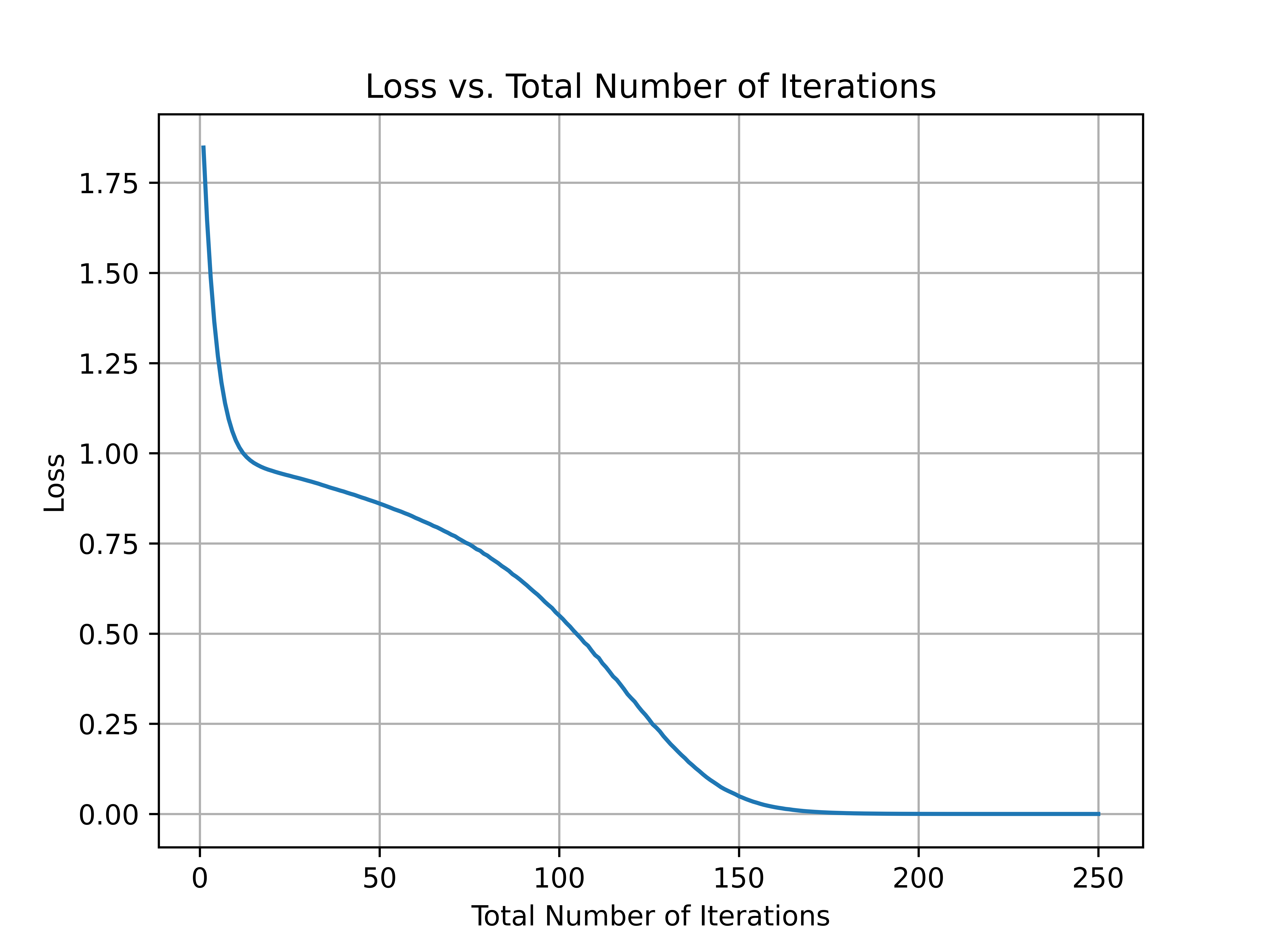Unsurprisingly, increasing the total number of iterations decreases the loss function even more. In a future blog post, I will use this model to analyze more interesting problems.

To see the python code that I wrote for this example, see here.