Using a Markov Decision Process to Model Life

Imagine that life is comprised of two states. In one state you are sad, and, in the other, you are happy. If you are sad, you can either remain sad or you can try to become happy. If you try to become happy, there is a risk of failing. Hence, if you fail, then you remain sad. If you are happy, then you can either remain happy or you can try to be even happier. Similarly, there is risk to trying to become happier since failure results in being sad.

In many aspects of life, there are these two states and similar actions that individuals choose. For example, consider when someone who has repeatedly used a product for a long time sees an ad of a potentially better product. Do they keep on using the product they have used for a long time or do they risk purchasing the newer product? Or consider when a worker that is unhappy with their current job faces a new job opportunity with better pay? Should they spend time applying for the new job or remain at their current firm? On the contrary, should a founder of a profitable company (in the happy state) ever abandon his company in order to try to start a new firm?

These are some of the many questions that I attempt to answer in this blog post. I create a Markov decision process (MDP) to model the randomness of the result of an action. Specifically, a player may choose some action whose result may not be deterministic. Hence, in game theory lingo, this is equivalent to having nature move after a player takes an action in a repeated game.

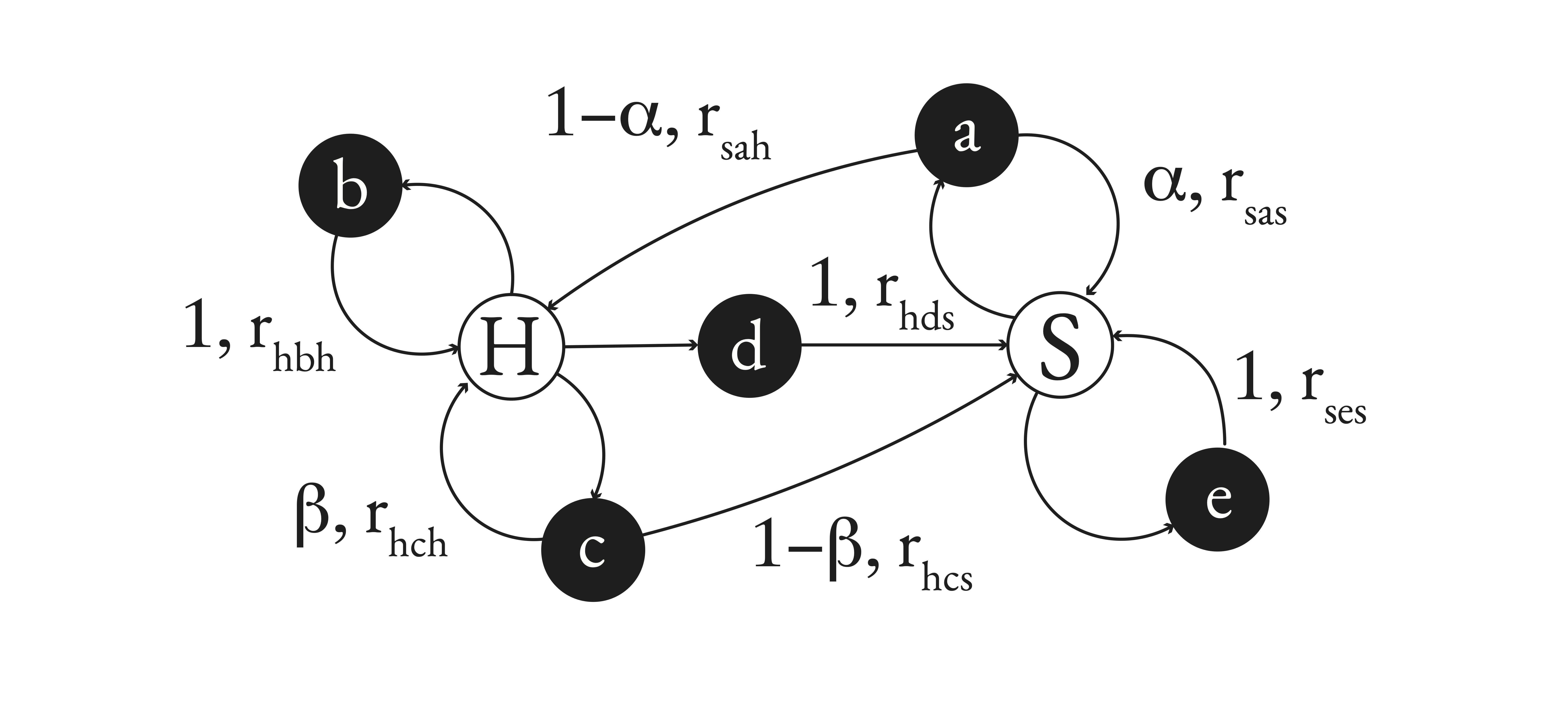
MDP Model of Life

I now define the important parameters and assumptions of the model. Let the set of actions $\mathcal{A}=\{a, b, c, d, e\}$ and let the set of states be $\mathcal{S}=\{S, H\}$. I abuse notation sometimes by writing $\mathcal{A}(s) \subseteq$ $\mathcal{A}$, which means the set of actions that are available at some state $s \in \mathcal{S}$. If the agent is at state $S$ and takes action $a$, then $\alpha$ is the probability that he ends up at state $S$ again. Likewise, if the agent is at state $H$ and takes action $c$, then $\beta$ is the probability that he ends up at state $H$ again. Hence, the probabilities $1-\alpha$ and $1-\beta$ model when the agent does not end up at $S$ or $H$ again, respectively. The reward $r_{i j k}$ is the reward received from starting at state $i \in \mathcal{S}$ and then taking action $j \in \mathcal{A}$ to end up at state $k \in \mathcal{S}$. $\gamma$ is a discount factor representing how much an agent values future rewards at some time. The diagram below is an illustration of these ideas.

Further, given a state $s \in \mathcal{S}$ and an action $a \in \mathcal{A}(s)$ to be taken at that state, the value of the state $v_a(s)$ is the expected value of the total returns now and over time of choosing such an action. This expected value accounts for the agent possibly retuming to the same state and other states after the optimal action.

The result by Bellman provides a straightforward method to find the optimal action or policy. See the seminal papers, (Bellman, 1952) and (Bellman, 1957), for more details on the existence and uniqueness of solutions. Following his work, in my model, let $v_*(s)$ be the optimal value at state $s \in \mathcal{S}$ when the optimal action is chosen. We then have

$\begin{array}{c} v_{*}(S)=\max \left\{\alpha\left(r_{sas}+\gamma v_{*}(S)\right)+(1-\alpha)\left(r_{sah}+\gamma v_{*}(H)\right), r_{ses}+\gamma v_{*}(S)\right\} \text { and } \\ v_{*}(H)=\max \left\{\beta\left(r_{hch}+\gamma v_{*}(H)\right)+(1-\beta)\left(r_{hcs}+\gamma v_{*}(S)\right), r_{hbh}+\gamma v_{*}(H), r_{hds}+\gamma v_*(S)\right\}. \end{array}$

Solving the optimal values at each state then identifies the optimal policies at each state.

An Example of the Model of Life

The equations above tell us a lot about how to think in different situations. If I am in the sad state $S$, depending on the rewards of all actions and the probabilities that I believe are associated with actions $a$ and $c$, my optimal action when I am sad could differ. Similarly, this idea can also be applied to when I am in the happy state.

For example, consider the case when a founder of a big firm decides whether to pursue a potentially market breaking idea (or product). He has three choices. The first choice is he does not pursue the idea and remains at his company earning him a reward of 2. The second option he has is to delegate the idea to another person and loan him money to start the venture. In this case, he risks losing the money with probability 0.8 and ending up with no job, in which case his reward is -2. If the other person succeeds, then his reward is 3. Now, his third option is to quit his job, yielding a reward of -2.

Now consider the case when he has no job and is working on his idea. He has two options under this scenario. The first is to continue to work on his idea, in which case he receives reward 0. The second option is to sell the product to the public. With probability 0.9, the idea is favorable when he pushes it to the market yielding a reward of 10. If the product does not sell well, his reward is -2. Suppose that he discounts future rewards at 0.8.

In this example, Bellman’s equations state that the founder should pursue the potentially market breaking idea by quitting his job and obtaining a reward of -2. He should then sell the product to the public even if the probability of success is 0.9.

My model and analysis can be made more complex by allowing the probabilities of resulting in a certain state after an action to be dependent on some history of actions. Further, more analysis can be done on the tradeoff between the probability that the product sold is favorable and the reward that must be gained when the product is successfully introduced to the market. But to keep my point brief, I stop here.

If you would like to see the Mathematica code that I wrote for the example above, see here.

References

1. Bellman, R. (1952). On the theory of dynamic programming. Proceedings of the National Academy of Sciences, 38(8), 716–719.
2. Bellman, R. (1957). A Markovian decision process. Journal of Mathematics and Mechanics, 679–684.